4. Running the programs
The software package uses five general codes:
DCIPF2D: performs 2D forward modelling for DC and IP data
DCINV2D: inverts DC potentials to recover a 2D conductivity model
IPINV2D: inverts IP data to recover a 2D chargeability model
This section discusses the use of these codes individually.
4.1. Introduction
All programs in the package can be executed under Windows or Linux environments. They can be run by typing the program name followed by a control file in the “command prompt” (Windows) or “terminal” (Linux). They can be executed directly on the command line or in a shell script or batch file. When a program is executed without any arguments, it will print the usage to screen.
4.1.1. Execution on a single computer
The command format and the control, or input, file format on a single machine are described below. Within the command prompt or terminal, any of the programs can be called using:
program \(arg_1\) [\(arg_2\) \(\cdots\) \(arg_i\)]
where:
program is the name of the executable
\(arg_i\) is a command line argument, which can be a name of corresponding required or optional file. Optional command line arguments are specified by brackets: . NOTE: Typing -inp as the control file, serves as a help function and returns all of the keyword combinations allowed for that program.
Each control file contains a formatted list of arguments, parameters, and file names in a combination specific for the executable, which can be in any order. Values that are being set by the user are given to each program through a specific list of keywords (e.g. WEIGHT, to specify the type of weighting). Different control file formats will be explained further in the document for each executable. All files are in ASCII text format - they can be read with any text editor. Input and control files can have any name the user specifies. Details for the format of each file can be found in Section Elements. When inputting a file, the word FILE should be following the keyword (e.g., MESH FILE mesh.msh). If a value is being used than the word VALUE will follow a keyword (e.g., COND VALUE 0.001).
4.2. DCIPF2D
This program performs forward modelling of DC and IP data. Command line usage:
dcipf2d dcipf2d.inp
where the input file, dcipf2d.inp, is described below. The options can be in any order.
4.2.1. Input files
Keywords for the input file dcipf2d.inp are:
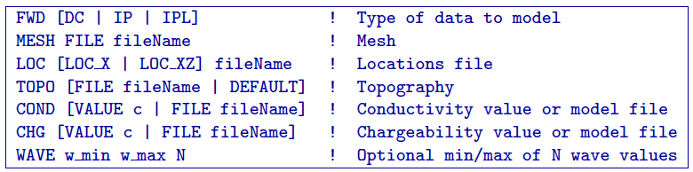
FWD: The choices after this keyword are:
DC for DC forward modelling. The chargeability model and wave, if given, is ignored for DC forward modelling only.
IP for IP forward modelling.
IPL for IP forward modelling using product of the sensitivity matrix and chargeability.
MESH FILE The 2D mesh file name is followed after these keywords. For example MESH FILE mesh.msh.
LOC The observation locations. The choices after this keyword are:
LOC_X when giving simple or surface locations formats.
LOC_XZ when using the general locations format.
TOPO The choices for the topography are:
FILE followed by the name of the topography file.
DEFAULT for flat topography at and elevation of 0.
COND The choices for the conductivity model are:
FILE followed by the name of the conductivity file .
VALUE followed by a number for the conductivity throughout the mesh.
CHG The choices for the chargeability model are:
FILE followed by the name of the chargeability file .
VALUE followed by a number for the chargeability throughout the mesh.
WAVE is followed by 3 constants: w_min, w_max and N. These are the wave numbers used in the cosine transform. There will be wave values, log spaced from to in time. The default values (if WAVE is not given) is w_min = 2.5e-4, w max = 1.0, and N= 13.
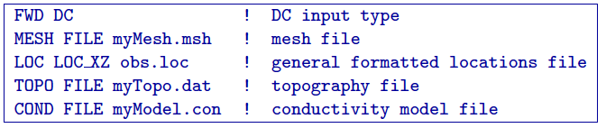
4.2.2. Example of dcipf2d.inp
Example of an input file for DCIPF2D to model DC data that are given in general format and a with a topography file:
4.2.3. Output files
The files created by DCIPF2D are:
obs_dc.dat The computed DC potential data.
obs_ip.dat The computed IP data if the option IP is chosen.
obs_ipL.dat The computed IP data if the option IPL is chosen.
4.3. DCINV2D
This program performs the inversion of DC resistivity data. Command line usage:
dcinv2d dcinv2d.inp
where the input file, dcinv2d.inp, is described below. The options can be in any order. The minimum keywords needed for an inversion are MESH and OBS.
4.3.1. Input Files
Keywords for the input file dcinv2d.inp are:
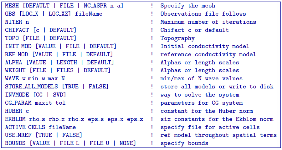
MESH The choices after this keyword are:
DEFAULT the programs creates a mesh (output dcinv2d.msh) with 3 cells between electrodes and the aspect ratio of the top cells set to 3. NOTE: This option assumes that the data are collected by commonly used arrays and that the topographic relief is moderate. Thus, this option may not be optimal when the data are collected with unusual electrode geometry or when data are collected over severe surface topography. In such cases, the user should redesign the mesh so that it is better suited for the particular needs of the data set.
FILE file name of the mesh
NC_ASPR n a creates a mesh (output dcinv2d.msh) that has n cells between the electrodes and the aspect ratio of the top cells is set to a.
OBS The observation locations. The choices after this keyword are:
LOC_X when giving simple or surface locations formats
LOC_XZ when using the general locations format.
NITER A value follows this keyword representing the number of maximum iterations for the inversion. NOTE: The program will terminate before the specified maximum number of iterations is reached if the expected data misfit is achieved and if the model norm has plateaued. However, if the program exits when the maximum iteration is reached, the file dcinv2d.out should be checked to see if the desired (based on the number of data and chi factor) has been reached and if the model norm is no longer changing. If either of these conditions has not been met then the program should be restarted. If the desired misfit level is not achieved, but the model norm has plateaued and the model is not changing between successive iterations, then the user may want to adjust the target misfit to a higher value. Also an investigation as to which data are most poorly fit can be informative. It may be that the assigned standard deviations to specific data are unrealistically small. The program restarts using the information in dcinv2d.out and dcinv2d.con.
CHIFACT The value at which the program reproduced the data. The choices after this keyword are:
DEFAULT where the program will start with 1e-3 initially and then when the misfit stop decreasing, the chi factor will be changed by 10%
constant the value to set the chi factor (1 is when the data misfit equals the number of data), or if a value is not there, but CHIFACT is given, the program will stop when the data misfit reaches the number of data
TOPO The choices after this keyword are:
FILE followed by the name of the topography file
DEFAULT for flat topography at an elevation of 0.
INIT_MOD The choices for the initial model are:
FILE filename name of the initial conductivity file
VALUE constant the value for the initial conductivity throughout the mesh
DEFAULT for the initial model to be set to the reference model.
REF_MOD The choices for the reference model are:
FILE filename name of the reference conductivity file
VALUE constant the value for the reference conductivity throughout the mesh
DEFAULT the reference model is equal to the best fitting half-space model.
WAVE is followed by 3 constants: w_min, w_max and N. These are the wave numbers used in the cosine transform. There will be wave values, log spaced from to in time. The default values (if WAVE is not given) is w_min = 2.5e-4, w max = 1.0, and N= 13.
ALPHA The choices after this keyword are:
DEFAULT where the program will set \(\alpha_s\) = 0.001*(90\(/\)max electrode separation)\(^2\) and \(\alpha_x = \alpha_z = 1\).
VALUE a_s a_y a_z the user gives the coefficients for the each model component for the model objective function from equation (2.11): \(\alpha_s\) is the smallest model component, \(\alpha_x\) is along line smoothness, and \(\alpha_z\) is vertical smoothness.
LENGTH L_x L_z the user gives the length scales and the smallest model component is calculated accordingly. The conversion from \(\alpha\)’s to length scales can be done by:
\[L_x = \sqrt{\frac{\alpha_x}{\alpha_s}} ; ~L_z = \sqrt{\frac{\alpha_z}{\alpha_s}}\]where length scales are defined in meters. When user-defined, it is preferable to have length scales exceed the corresponding cell dimensions.
WEIGHT The weighting for the model objective function allows for three options:
DEFAULT No weighting is supplied (all values of weights are 1)
FILE filename The weighting is supplied as a file with all the weights in one file
FILES fileS fileX fileZ The weighting is supplied as three separate weight files with the weight for the smallest model component in fileS, the x-component written in file fileX and the z-component written in fileZ.
STORE ALL MODELS There are two choices:
TRUE Write all models and predicted data to disk. Each iteration will have dcinv2d_xx.con and dcinv2d_xx.pre files where xx is the iteration (e.g., 01 for the first iteration)
FALSE Only the final model and predicted data file are written. These files are named dcinv2d.con and dcinv2d.pre for the conductivity and predicted data, respectively.
INVMODE This specifies the way the system is solved:
SVD Solve the system using a subspace method with basis vectors. This is the solution methodology of the original code and the default if not given.
CG Solve the system using a subspace method with conjugate gradients (CG). This allows additional constraints (i.e., Huber and Ekblom norms) to be incorporated into the code.
CG_PARAMS is used when the inversion mode is . The keyword is followed by two constants: maxit specifying the maximum number of iterations (default is 10), and tol specifying the solution’s accuracy (default is 0.01)
HUBER The Huber norm is used when evaluating the data misfit. A constant follows this keyword and this option is only available when using the CG inversion mode option. The default value is 1e100. The constant c is from equation (2.10).
EKBLOM Use the Ekblom norm. Six (6) values should follow this keyword: \(\rho_s; \rho_x; \rho_z; \varepsilon_s; \varepsilon_x; \varepsilon_z\) representing the constants found in equation :eq:ekblom`.
ACTIVE_CELLS followed by the file name of the active cell file.
USE_MREF This option is used to decide if the reference model should be in the spatial terms of the model objective function (equation (2.11)). There are two options: TRUE to include the reference model in the spatial terms or FALSE to have the reference model only in the smallest model component.
BOUNDS The bounds options are:
NONE Do not include bounds in the inversion
VALUE lwr upr Give a constant global lower bound of lwr and upper bound of upr.
FILE_L fileName The lower bound is given in a file and is in the model format.
FILE_U fileName The upper bound is given in a file and is in the model format.
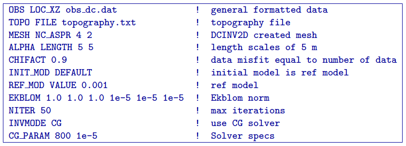
4.3.2. Example of dcinv2d.inp
Below is an example of the input file dcinv2d.inp. The code will create a mesh with 4 cell between electrode locations and the aspect ratio of the size top cells set to 2. This means the reference and initial models will not be given in a file, but rather set to 0.001 S/m. The length scales will be 5 m in each direction and the Ekblom norm will have exponents of 1.0 in each direction to emphasize blockiness. It will start from scratch and stop after 50 iterations if the desired misfit (equal to 90% of the number of data) is not achieved. Conjugate gradients are used to solve the system of equations with a maximum number of CG iterations set at 800 and a relative accuracy of 1e-5. There are no bounds in this inversion.
4.3.3. Output Files
DCINV2D will create the following files:
dcinv2d.log The log file containing the minimum information for each iteration, summary of the inversion, and standard deviations if assigned by DCINV2D.
dcinv2d.out The developers log file containing the values of the model objective function value(\(\psi_m\)), trade-off parameter (\(\beta\)), and data misfit (\(\psi_d\)) at each iteration
dcinv2d_iter.con Conductivity model for each iteration (iter defines the iteration step) if is used
dcinv2d_iter.pre Predicted data for each iteration (iter defines the iteration step) if is used
dcinv2d.pre Predicted data file that is updated after each iteration (will also be the final predicted data)
dcinv2d.con Conductivity model that matches the predicted data file and is updated after each iteration (will also be the final ecovered model)
sensitivity.txt Model file of average sensitivity values for the mesh
4.4. IPINV2D
This program performs the 2D inversion of induced polarization data. Command line usage:
ipinv2d ipinv2d.inp
for the control ipinv2d.inp described below. The options can be in any order. The minimum keywords needed for an inversion are MESH, OBS, and COND.
4.4.1. Input Files
Keywords for the input file ipinv2d.inp are:
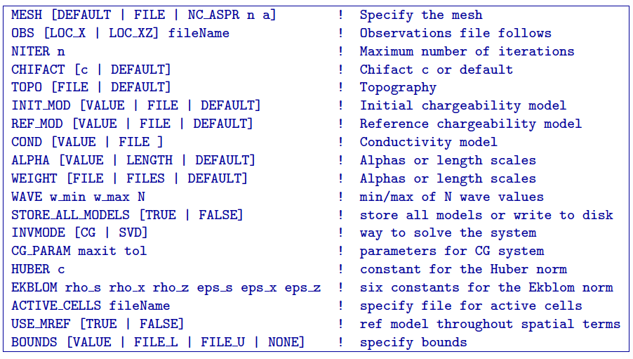
MESH The choices after this keyword are:
DEFAULT the programs creates a mesh (output dcinv2d.msh) with 3 cells between electrodes and the aspect ratio of the top cells set to 3. NOTE: This option assumes that the data are collected by commonly used arrays and that the topographic relief is moderate. Thus, this option may not be optimal when the data are collected with unusual electrode geometry or when data are collected over severe surface topography. In such cases, the user should redesign the mesh so that it is better suited for the particular needs of the data set.
FILE file name of the mesh
NC_ASPR n a creates a mesh (output dcinv2d.msh) that has n cells between the electrodes and the aspect ratio of the top cells is set to a.
OBS The observation locations. The choices after this keyword are:
LOC_X when giving simple or surface locations formats
LOC_XZ when using the general locations format.
NITER A value follows this keyword representing the number of maximum iterations for the inversion. NOTE: The program will terminate before the specified maximum number of iterations is reached if the expected data misfit is achieved and if the model norm has plateaued. However, if the program exits when the maximum iteration is reached, the file ipinv2d.out should be checked to see if the desired (based on the number of data and chi factor) has been reached and if the model norm is no longer changing. If either of these conditions has not been met then the program should be restarted. If the desired misfit level is not achieved, but the model norm has plateaued and the model is not changing between successive iterations, then the user may want to adjust the target misfit to a higher value. Also an investigation as to which data are most poorly fit can be informative. It may be that the assigned standard deviations to specific data are unrealistically small. The program restarts using the information in ipinv2d.out and ipinv2d.con.
CHIFACT The value at which the program reproduced the data. The choices after this keyword are:
DEFAULT where the program will start with 1e-3 initially and then when the misfit stop decreasing, the chi factor will be changed by 10%
constant the value to set the chi factor (1 is when the data misfit equals the number of data), or if a value is not there, but CHIFACT is given, the program will stop when the data misfit reaches the number of data
TOPO The choices after this keyword are:
FILE followed by the name of the topography file
DEFAULT for flat topography at an elevation of 0.
INIT_MOD The choices for the initial model are:
FILE filename name of the initial chargeability file
VALUE constant the value for the initial chargeability throughout the mesh
DEFAULT for the initial model to be set to the reference model.
REF_MOD The choices for the reference model are:
FILE filename name of the reference chargeability file
VALUE constant the value for the reference chargeability throughout the mesh
DEFAULT the reference model is equal to 0.
COND The choices for the conductivity model (required) are:
FILE filename name of the conductivity file
VALUE constant the value for the conductivity throughout the mesh. NOTE: The conductivity of a uniform half space for IP inversions should only be used for preliminary examination of the data. When there is little structure in the background conductivity, the inversion using this default mode can yield a reasonable chargeability model and it is justifiable to fit the data close to the expected misfit value. However, when the background conductivity deviates greatly from a uniform half space, reproducing the data to within the assumed errors will certainly result in over-fitting the data. If the half-space conductivity is assumed, then it is prudent to assign a value greater than 1.0 for chi factor when the background conductivity is structurally complex. The judgment can be made based upon the complexity of the apparent resistivity pseudo-section.
WAVE is followed by 3 constants: w_min, w_max and N. These are the wave numbers used in the cosine transform. There will be wave values, log spaced from to in time. The default values (if WAVE is not given) is w_min = 2.5e-4, w max = 1.0, and N= 13.
ALPHA The choices after this keyword are:
DEFAULT where the program will set \(\alpha_s\) = 0.001*(90\(/\)max electrode separation)\(^2\) and \(\alpha_x = \alpha_z = 1\).
VALUE a_s a_y a_z the user gives the coefficients for the each model component for the model objective function from equation (2.11): \(\alpha_s\) is the smallest model component, \(\alpha_x\) is along line smoothness, and \(\alpha_z\) is vertical smoothness.
LENGTH L_x L_z the user gives the length scales and the smallest model component is calculated accordingly. The conversion from \(\alpha\)’s to length scales can be done by:
\[L_x = \sqrt{\frac{\alpha_x}{\alpha_s}} ; ~L_z = \sqrt{\frac{\alpha_z}{\alpha_s}}\]where length scales are defined in meters. When user-defined, it is preferable to have length scales exceed the corresponding cell dimensions.
WEIGHT The weighting for the model objective function allows for three options:
DEFAULT No weighting is supplied (all values of weights are 1)
FILE filename The weighting is supplied as a file with all the weights in one file
FILES fileS fileX fileZ The weighting is supplied as three separate weight files with the weight for the smallest model component in fileS, the x-component written in file fileX and the z-component written in fileZ.
STORE ALL MODELS There are two choices:
TRUE Write all models and predicted data to disk. Each iteration will have ipinv2d_xx.con and ipinv2d_xx.pre files where xx is the iteration (e.g., 01 for the first iteration)
FALSE Only the final model and predicted data file are written. These files are named ipinv2d.con and ipinv2d.pre for the chargeability and predicted data, respectively.
INVMODE This specifies the way the system is solved:
SVD Solve the system using a subspace method with basis vectors. This is the solution methodology of the original code and the default if not given.
CG Solve the system using a subspace method with conjugate gradients (CG). This allows additional constraints (i.e., Huber and Ekblom norms) to be incorporated into the code.
CG_PARAMS is used when the inversion mode is . The keyword is followed by two constants: maxit specifying the maximum number of iterations (default is 10), and tol specifying the solution’s accuracy (default is 0.01)
HUBER The Huber norm is used when evaluating the data misfit. A constant follows this keyword and this option is only available when using the CG inversion mode option. The default value is 1e100. The constant c is from equation (2.10).
EKBLOM Use the Ekblom norm. Six (6) values should follow this keyword: \(\rho_s; \rho_x; \rho_z; \varepsilon_s; \varepsilon_x; \varepsilon_z\) representing the constants found in equation :eq:ekblom`.
ACTIVE_CELLS followed by the file name of the active cell file.
USE_MREF This option is used to decide if the reference model should be in the spatial terms of the model objective function (equation (2.11)). There are two options: TRUE to include the reference model in the spatial terms or FALSE to have the reference model only in the smallest model component.
BOUNDS The bounds options are:
NONE Do not include bounds in the inversion
VALUE lwr upr Give a constant global lower bound of lwr and upper bound of upr.
FILE_L fileName The lower bound is given in a file and is in the model format.
FILE_U fileName The upper bound is given in a file and is in the model format.
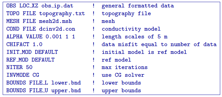
4.4.2. Example of ipinv2d.inp
Below is an example of the input file ipinv2d.inp. The code reads mesh dcinv2d.msh from the file with topography from topography.txt. The means the reference and initial models will be set to one another and equal zero. The conductivity model is given as the output from . The alpha values have been given for \(\alpha_s=0.001\) and \(\alpha_x = \alpha_z = 1\) . The model objective function will have an \(l_2\) norm (which would also be the same as EKBLOM 2 2 2 epsS epsX epsZ). It will start from scratch and stop after 50 iterations if the desired misfit (equal to the number of data) is not achieved. Conjugate gradients are used to solve the system of equations and the bounds are given in two separate files.
4.4.3. Output Files
IPINV2D will create the following files:
ipinv2d.log The log file containing the minimum information for each iteration, summary of the inversion, and standard deviations if assigned by IPINV2D.
ipinv2d.out The developers log file containing the values of the model objective function value(\(\psi_m\)), trade-off parameter (\(\beta\)), and data misfit (\(\psi_d\)) at each iteration
ipinv2d_iter.chg Chargeability model for each iteration (iter defines the iteration step) if is used
ipinv2d_iter.pre Predicted data for each iteration (iter defines the iteration step) if is used
ipinv2d.pre Predicted data file that is updated after each iteration (will also be the final predicted data)
ipinv2d.chg Chargeability model that matches the predicted data file and is updated after each iteration (will also be the final recovered model)
sensitivity.txt Model file of average sensitivity values for the mesh