6.2. DC Inversion of the forward model
The goal of this section is to illustrate the performance of the inversion program when different combinations of input parameters are used. We have carried out nine DC inversions of the simulated DC data presented in the Forward section.
6.2.1. DC Inversion: All default
First, the synthetic data were inverted using the all-default option:
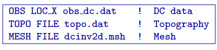
In this file, the first line indicates that the data file (obs_Uncert_5pc_0p001V.dc) is of surface format. The second line contains the reference to topography file (TOPO.DAT). The third line is in reference to the mesh file (dcinv2d.msh). If there is no topography it is not necessary to include either the mesh, or the topography file in all-default mode. will construct a mesh in automatic mode and consider topography to be zero. In our case we have user-defined topography and mesh file is provided. The result of the all-default inversion is shown in Figure Fig. 6.6. The best fitting half space was approximately 120 ohm-m.
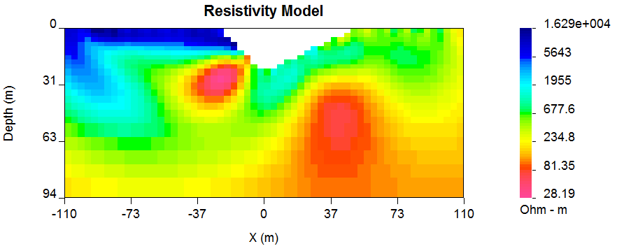
Fig. 6.6 Inversion of synthetic DC data using all-default mode.
6.2.2. DC Inversion: CG solution using a constant reference model
In the next example, definition of some parameters has been set to user-defined and changed. In real life this can be done if there is a higher level of certainty regarding some starting parameters (prior information). The control file for the next example is provided below:
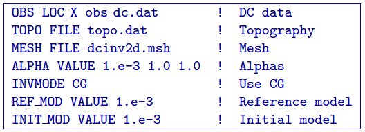
In this example, the fourth line indicates that the smallness coefficient (\(\alpha_s\)) is now user-defined (set to 0.001). The fifth line means that the system solver has been switched from default (Singular Value Decomposition or SVD solver) to the Conjugate Gradient solver (CG). The reference model has been set to 0.001 S/m (or 1000 Ohm m). The initial model has been set to the same as reference model. The results of applying these control file parameters are shown in the inversion model in Figure Fig. 6.7.
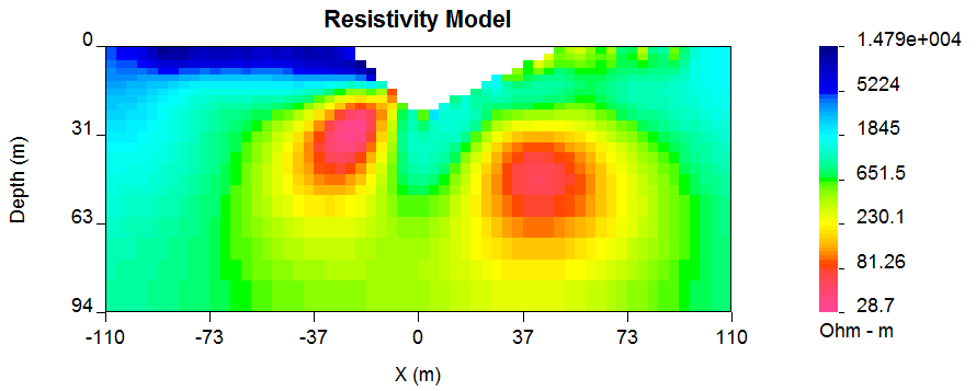
Fig. 6.7 Inversion of synthetic DC data using user-defined smallness parameter (\(\alpha_s\)s) 1000 Ohm m half space as both: reference and a starting model.
The basic features of the models in Figure Fig. 6.6 and Figure Fig. 6.7 are similar. Both conductors have been located and so has the resistive overburden on the left. (Compare with the synthetic model in Figure Fig. 6.2). Nevertheless, there are differences. Figure Fig. 6.7, which uses a more resistive reference model, supports the interpretation of closure for the body on the right. There is also an odd structure emanating from the left most part of the resistive overburden observed in Figure Fig. 6.6 that is not observed in Figure Fig. 6.7. The primary differences between the two models can be explained through the use of a DOI (Depth of Investigation) plot. For the present we use Figure Fig. 6.7 as a reference and Figure Fig. 6.6 as an additional model.
When the inversion volume is cut with respect to the DOI, then differences in the images are no longer so apparent. For the remainder of the example section we shall use the reference the model described in Figure Fig. 6.7 (1000 Ohm m half space) as the default model.
6.2.3. Depth of Investigation (DOI)
Models produced by inversion of DC resistivity data tend to approach the background conductivity of the reference model. At those depths the recovered model is no longer being influenced by the data. We can use this result to help estimate our depth of investigation. If there are at two reasonable models obtained using different reference models, the two models can be compared to identify which regions of the model are most significantly affected by the measurements. The results of doing this are explained next.
Using DCIP2D, the method is applied within the DCIP2D-MODEL-VIEWER GUI, using Depth of investigation option in the menu. There must be a second model that was recovered using the same mesh as the one being observed. Any two different inversions results can be used. Here we use 1000 Ohm-m halfspace as our best model and we want blank out those sections of the model that are not well controlled by the data. A second inversion using a background of 106 Ohm-m (the default value from the code) and used that to compute the DOI. In Figure Fig. 6.8 (a-b) shows the model with cutoffs of 0.1 and 0.4.
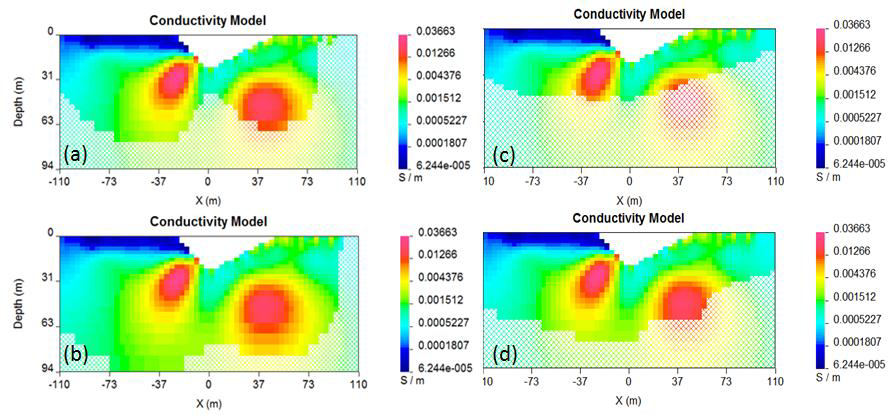
Fig. 6.8 Assessing the depth of investigation (DOI): (a) based on recovered model (cut-off=0.1), (b) based on recovered model (cut-off = 0.4), (c) based on sensitivity (cut-off = 0.5), and (d) based on sensitivity (cut-off = 0.6).
Another option to assess the depth of investigation is through the analysis of the sensitivities. In DCIP2D there is a capability to visualize the sensitivities using the DCIP2D-MODEL-VIEWER GUI (Figure Fig. 6.8 c and Figure Fig. 6.8 d). Generally, the lower sensitivities correspond to less reliable model parameters (deeper-seated cells); higher sensitivities correspond to those model cells, which have most effect on the data (usually closer to surface). A good way to assess the DOI is by plotting the model on the full mesh extent (including the padding cells, Figure 19). In this figure we use the DOI evaluated from 1000 and 106 Ohm-m half spaces (that is, the same as Figure Fig. 6.8 a) and Figure Fig. 6.8 b). As the DOI threshold decreases we limit the region of the model to that which is most controlled by the data. See (Figure Fig. 6.9 a-c). The final choice of cutoff is selected by the user.
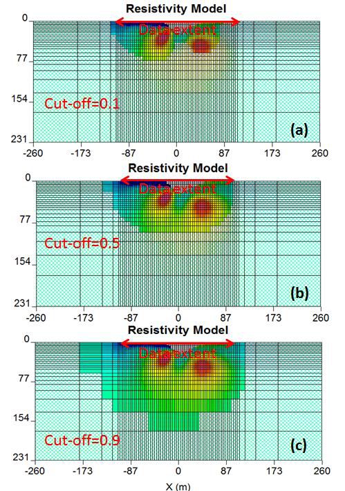
Fig. 6.9 Assessing the depth of investigation (DOI): (a) based on recovered model (cut-off=0.1), (b) based on recovered model (cut-off = 0.4), (c) based on sensitivity (cut-off = 0.5), and (d) based on sensitivity (cut-off = 0.6).
6.2.4. DC Inversion: Non-uniform reference model
The next example is very similar to the previous inversion, with an exception that a different reference model is introduced (Figure Fig. 6.10). As opposed to the previous example, where the reference model was set to a 1000 Ohm m half space, the new model includes an elongated conductive (10 Ohm m) rectangular block. The elongated block has the same value as the conductivity anomaly but the boundaries do not coincide. Moreover the block in the true model has smoothed boundaries. In summary, the supplied reference model has captured some aspects of the true conductivity but it is not an exact reflection of what is there. This example has been contrived to illustrate what happens with the options of including, or omitting, the reference model in derivative terms in the objective function according to equations (2.13) and (2.16).
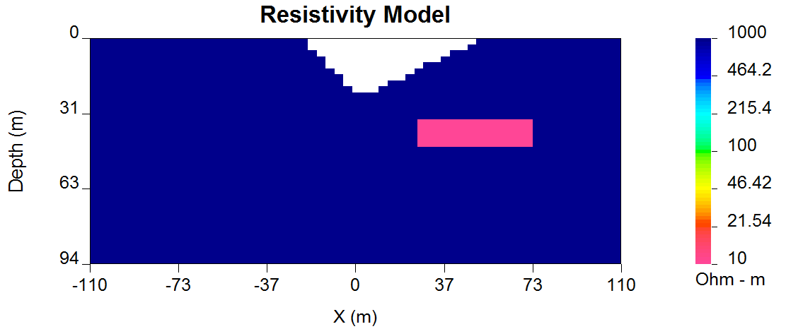
Fig. 6.10 Reference model applied for the synthetic example illustration.
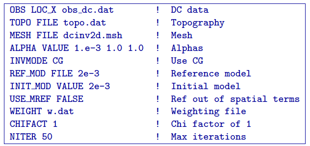
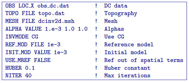
In the first example (control file provided below) the reference model was used in only the smallest model component.
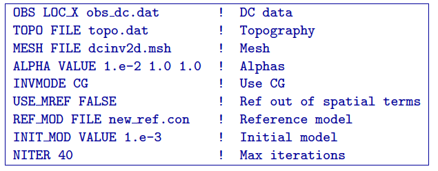
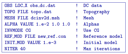
In this control file line 7 now indicates that the reference model should be read from a file, rather than assigned a constant value; line 6 indicates that the reference model should be defined in non-derivative terms and line 9 is indicating that the maximum number of iterations for this inversion should not exceed 40. The results of this inversion can be seen in Figure Fig. 6.11.
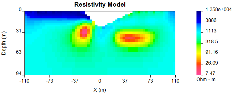
Fig. 6.11 Reference model applied for the synthetic example illustration.
This is a superior model compared to that in Figure Fig. 6.7. The magnitude of the conductive anomaly is much better recovered, although at 7.6 Ohm-m it is slightly less resistive than the true value of 10 Ohm-m. It has a well-defined elongated shape with steep gradational boundaries that are good representations of the true model. If we are more confident in the locations of the boundaries of the block in the reference model, then this can be incorporated into the inversion. We next carry out an inversion in which the reference model is included in the derivative terms. Below is the control file used for this inversion.
The line (USE_MREF_FALSE) from the previous example has been eliminated, switching the inversion into the default mode (reference model is defined in the derivative terms in default mode). This line also could have been changed to USE_MREF_TRUE).
The result is shown in Figure Fig. 6.12 and it produces a model that has boundaries at the same location as the reference block and there is even more over-shoot of the conductivity. For this example however, putting in the reference model into the derivative terms is stronger information than is justified. In most cases, the previous solution, where the reference model was left out of the derivative terms is preferable.
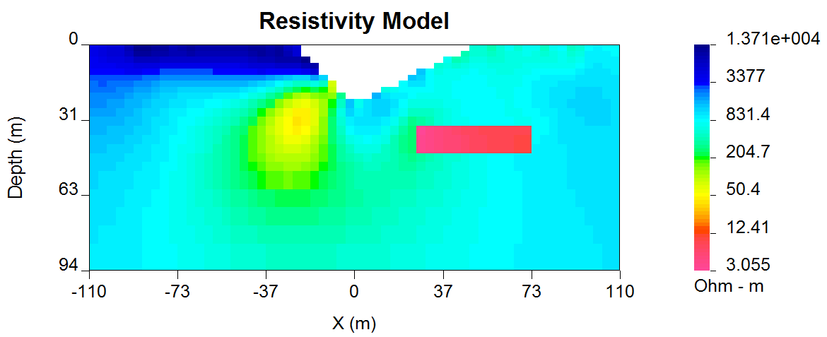
Fig. 6.12 Reference model applied for the synthetic example illustration.
This is not always the case. Consider a situation where the goal is to find a body beneath an overburden layer. The model and the reference model are shown in Figure Fig. 6.13. It might be supposed that information about the overburden thickness and its resistivity have been obtained through drilling. Two inversions are carried out. In the first (Figure Fig. 6.14 a) the reference model is omitted from the derivative term and the overburden boundary is characterized by a smooth transition. In the second case (Figure Fig. 6.14 b) the reference model is included in the derivative terms and the result is a cleaner delineation of the overburden and better definition of the sought body.
Fig. 6.13 A conductive block underneath the overburden: (a) the true model and (b) the reference model.
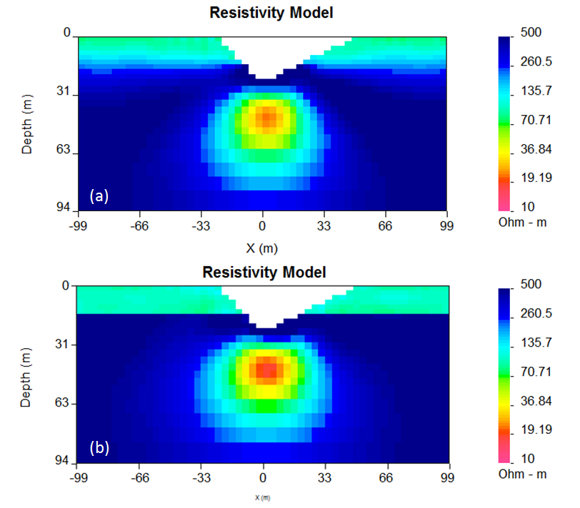
Fig. 6.14 Inversion results when (a) the reference model is not included in the derivative terms and when (b) the reference model is defined in derivative terms.
6.2.5. DC Inversion: Incorporating inactive cells constraint
In the next example it is illustrated how drilling data can be incorporated in the inversion using fixed cells constraint. In this example, the reference model has been set to the same elongated conductive block model as shown in Figure Fig. 6.13. The difference is that in this case additional information has been incorporated by fixing some reference model cell values. The values are taken from the reference model file (ref_new.con) but their values are fixed using active cells file (ACTIVE_CELLS active.txt), defined in line 6 of the control file provided below.
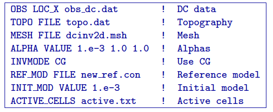
The active file format was previously discussed within the subsection Model in the section of the manual, however another example is provided below:
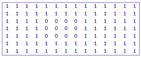
The format of this file is consistent with the model file, and the values equal to 1 define the model cells marked as active, while values equal to 0 define the model cells marked as inactive(without the capability affect the neighbouring cells). The case when inactive cells do not influence their neighbours is shown in Figure Fig. 6.15.
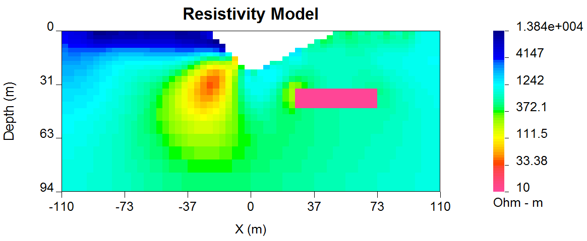
Fig. 6.15 Recovered model when the reference model cells are inactive and they do not influence the neighbouring cells.
If it is desired to have the inactive cells influence the values of neighboring cells, then their values are set to -1 as in the file below. The resultant inversion model is shown in Figure Fig. 6.16. The region of high conductivity has been extended away from the reference model and the anomaly smoothly transitions to the background.
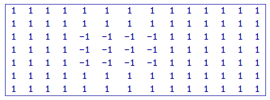
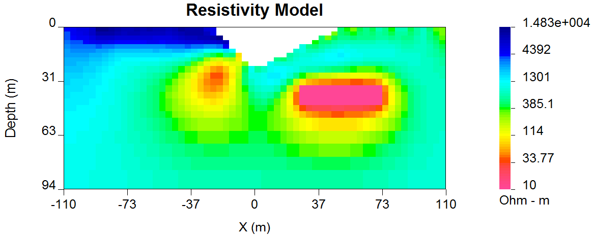
Fig. 6.16 Recovered model when cells are inactive, but their values influence those of the neighbouring cells.
6.2.6. DC inversion: Using weighting functions
The next example illustrates the situation when prior information is incorporated using the weighting function file. The synthetic model for this example is the same as illustrated in Figure Fig. 6.13. Instead of reference model, a weigthing file was used. The control file used for this inversion is shown below. The reference to the weighting file is provided in line 11 (WEIGHT W.dat).
The recovered model is illustrated in Figure Fig. 6.17 and is very similar to the model shown in Figure Fig. 6.14 b. The alternative of using a weighting file instead of the reference model facilitated the technical implementation of the prior constraints and brings an additional degree of freedom in being able to adjust the level of certainty in the a priori information by editing the weighting coefficients. In our case, the weighting coefficients were edited for the \(\boldsymbol{\vec{W}}_z\) matrix, where the sixth interface (corresponding to the bottom of the overburden) was set to 0.1 (as opposed to default weights of 1.0).
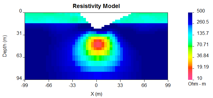
Fig. 6.17 Recovered model from the inversion using weighting file
6.2.7. DC Inversion: Using the Huber norm for data misfit
The next example illustrates the effects that large data errors can have on the inversion and how these can be ameliorated with the Huber norm. The data are the same as used in previous examples except that 5 data have been severely perturbed. The inversions are carried out with the same standard deviation estimates, as used previously, a 1000 ohm-m background, and a data file contaminated with bad apparent resistivity values. Figure Fig. 6.18 shows the contamination introduced to the apparent resistivity file used for the inversions.
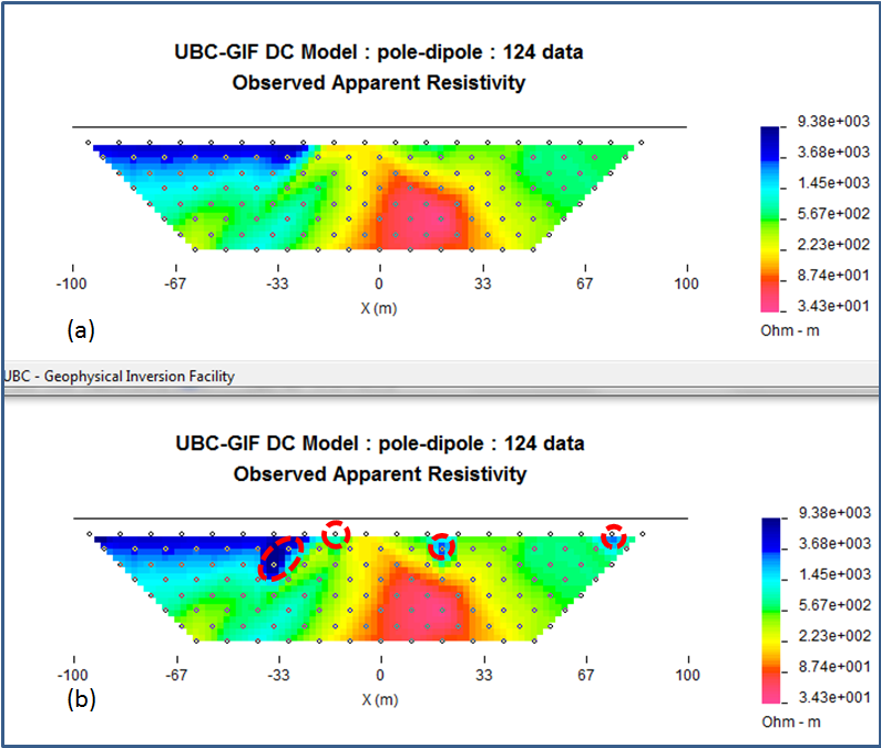
Fig. 6.18 The (a) true data and (b) data contaminated with noise that will be inverted.
The contaminated data were inverted using a standard \(l_2\) norm for the data misfit. The control file for this inversion is provided below:
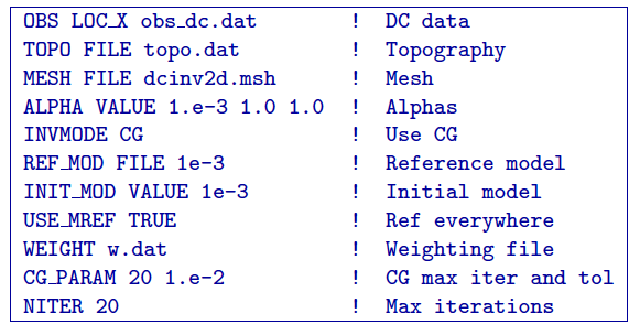
The results of the inversion are shown in Figure Fig. 6.19. The inversion ran for 20 iterations and the target misfit was not achieved and there were many artifacts. The reason is that the great effort was being made to fit the five erroneous data.
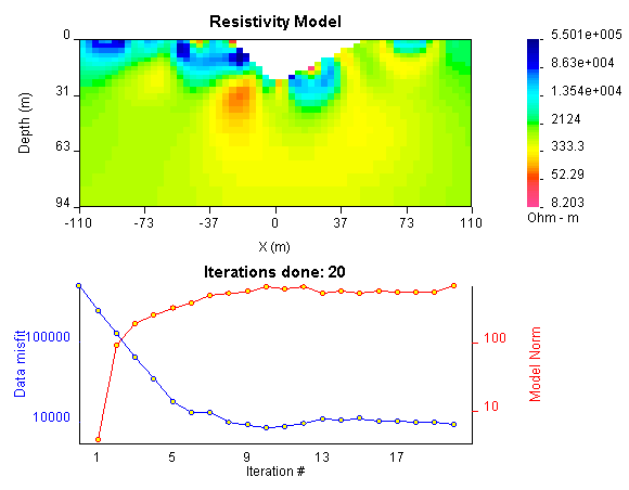
Fig. 6.19 Recovered model (top) and conversion curves (bottom) from the inversion of the contaminated data. The data misfit utilized an \(l_2\) norm.
In Figure Fig. 6.20 we show the observed data and the normalized misfit. Three of the five outliers are distinct and they contribute a value of 2067.05 to the final misfit of 9303. By recognizing them as outliers, they might be winnowed from further analysis but two erroneous data have been over fit by the modeling and as a result produced incorrect structure. This has led to other, higher quality data, having large misfits. This is characteristic of non-robust norms.
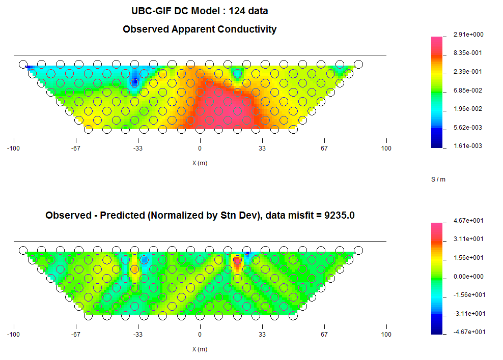
Fig. 6.20 Observed data (top) and the normalized difference (bottom) from the inversion using an \(l_2\) misfit measure.
In order to combat the effect that outliers in the data file may have on fitting the data using the \(l_2\) measure, Huber norm was imposed on the data fit. The example of the control file with Huber norm is shown below:
Line 9 in this control file has been set to so that all normalized data misfits with value greater than 0.1 will be evaluated with the \(l_1\) measure. The results are shown in Figure Fig. 6.21 and they appear much better, than in previous case. Nevertheless, they can still be improved by recognizing the existence of the highly erroneous data and winnowing them from the inversion. incorrect structure. This has led to other, higher quality data, having large misfits. This is characteristic of non-robust norms. Although the recovery is far from perfect, the main conductor bodies are now shown with satisfactory detail, comparing to the \(l_2\) normalization.
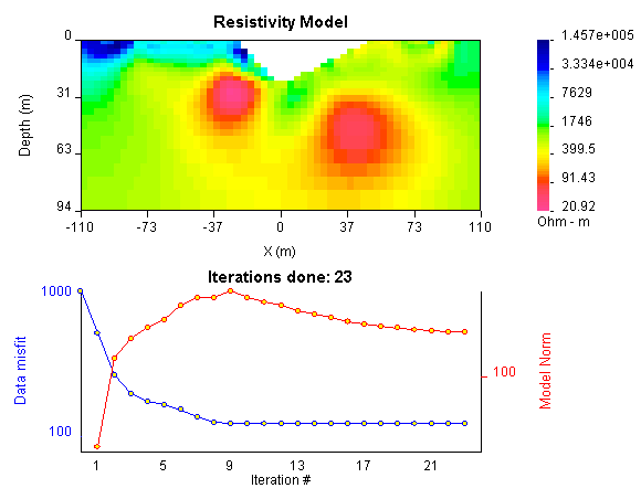
Fig. 6.21 (top) The recovered model from inversion of contaminated data using Huber norm for the data misfit and (b) the convergence curves.