6.3. IP Inversion of the forward model

The inversion of IP data is almost identical to the inversion of DC resistivity data. The primary difference is that IP is a linear problem and the forward modeling matrix is the sensitivity matrix from the DC resistivity inversion. The IP inversion code has the same functionality as the DC resistivity code and the control lines are identical. One essential difference is that positivity is strictly enforced in the IP inversion. IP data can be negative but the intrinsic chargeability is always positive. There is no need to repeat all of the inversions done for the DC. Rather, we will invert only a few examples to illustrate the algorithm.

The inversion of IP data is almost identical to the inversion of DC resistivity data. The primary difference is that IP is a linear problem and the forward modeling matrix is the sensitivity matrix from the DC resistivity inversion. The IP inversion code has the same functionality as the DC resistivity code and the control lines are identical. One essential difference is that positivity is strictly enforced in the IP inversion. IP data can be negative but the intrinsic chargeability is always positive. There is no need to repeat all of the inversions done for the DC. Rather, we will invert only a few examples to illustrate the algorithm.

The examples were designed to replicate the capabilities of DCIP2D, shown using the DC examples. The conductivity models used for IP inversions were mainly those, acquired from the corresponding DC inversions.

6.3.1. IP inversion: Zero-chargeability reference model

The first example was carried out using zero-chargeability reference half space and the conductivity model acquired from inverting the dc resistivity with 1000 Ohm-m half space reference. The control file for this inversion is shown below:

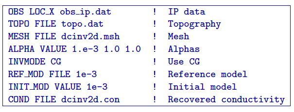
On the last line of this control file, there is the reference to the conductivity file, an essential input parameter for an IP inversion. This file has to come from a corresponding DC inversion, carried out prior to the IP inversion. The results of this inversion are shown in Figure Fig. 6.22.

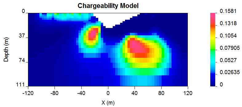
Fig. 6.22 Recovered chargeability model for a zero chargeability reference model and 1000 Ohm-m conductivity model.

6.3.2. IP inversion: Non-uniform reference model

In the next example, similarly to the DC inversions, we have introduced a chargeable block into the reference model (Figure Fig. 6.23).

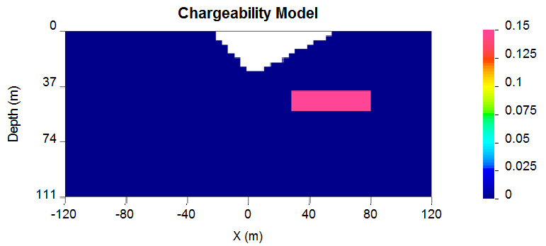
Fig. 6.23 The reference model applied to the synthetic example for illustration.

Further, the new reference model was introduced in the inversion and omitted from the derivative terms. The control file for the inversion is virtually identical as in case with analogous inversion of the DC data and is provided below. The resulting inversion is shown in Figure Fig. 6.24.

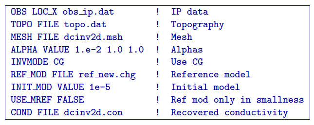
Fig. 6.24 Recovered model from IP inversion using the non-uniform reference model in the smallness term.

6.3.3. IP inversion: Using Ekblom measure to recover a blocky model

In this next example, the geological information is incorporated in the model objective function using the \(l_1\) norm measure rather than the default \(l_2\) norm. This allows recovery of a blocky model. The control file for this example is provided below, and the resultant inversion model is shown in Figure Fig. 6.25.

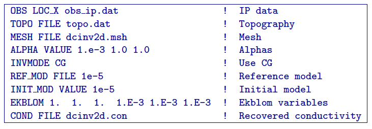
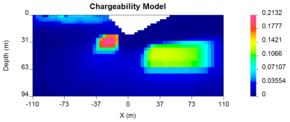
Fig. 6.25 Recovered model from IP inversion Using \(l_1\) measure (Ekblom norm) of model norm to recover a blocky model.

The resultant models are blocky and the central block has better defined boundaries than the deep block on the right. This arises because the right hand block is located close to the edge of the depth of investigation for the survey. To illustrate this we superpose the depth of investigation inferred by using the sensitivity function with a cutoff of 0.5. This is shown in Figure Fig. 6.26 to illustrate the depth of investigation (DOI) the model has been plotted on a larger scale.

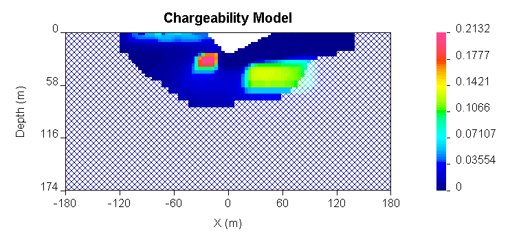
Fig. 6.26 The depth of investigation (DOI) for the IP inversion with an \(l_1\) model norm.

6.3.4. IP inversion: Reference model with inactive cells

This next example illustrates an inversion with a reference model with fixed cells (inactive). In this example, the inactive cells are representing a scenario when our constraints are acquired by incorporating borehole information. Out synthetic borehole is located on the profile at \(x=60\) (Figure Fig. 6.27 a). This reference model is now different and involves only the knowledge we have from the borehole data (Figure Fig. 6.27 b). The inversion was carried out in the mode, when the inactive cells may influence their neighbours and resulted in the chargeability distribution shown in Figure Fig. 6.27 c. In this mode the inversion extends the chargeability of the fixed cells away from the reference block. The case is very similar to the analogous example shown in the DC inversion. The control file used for this inversion is provided below:

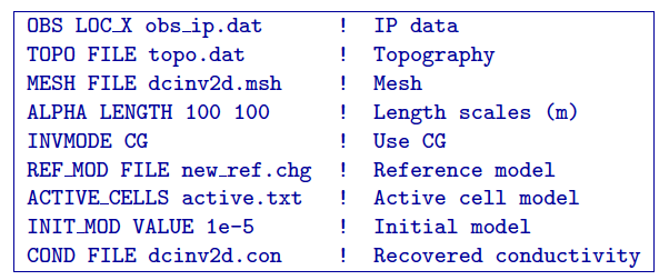
The active file is shown below, the structure has been edited so that two cells (one in each direction) around the synthetic borehole are set inactive and with the capability to influence the neighbours (i.e., -1)

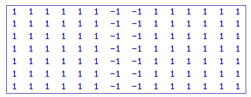
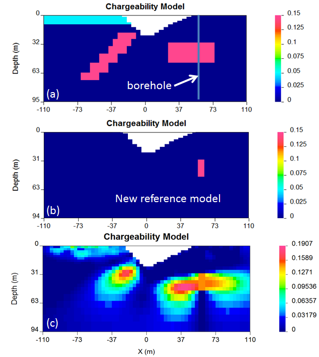
Fig. 6.27 (a) The true chargeability model with the borehole location. (b) The new reference model created from the borehole information. (c) Recovered model with the borehole locations set to inactive with influence (-1) on neighbouring cells.